Spatial lag model trees
Citation
Martin Wagner, Achim Zeileis (2019). “Heterogeneity and Spatial Dependence of Regional Growth in the EU: A Recursive Partitioning Approach.” German Economic Review, 20(1), 67-82. doi:10.1111/geer.12146 [ pdf ]
Abstract
We use model-based recursive partitioning to assess heterogeneity of growth and convergence processes based on economic growth regressions for 255 European Union NUTS2 regions from 1995 to 2005. Spatial dependencies are taken into account by augmenting the model-based regression tree with a spatial lag. The starting point of the analysis is a human-capital-augmented Solow-type growth equation similar in spirit to Mankiw et al. (1992, The Quarterly Journal of Economics, 107, 407-437). Initial GDP and the share of highly educated in the working age population are found to be important for explaining economic growth, whereas the investment share in physical capital is only significant for coastal regions in the PIIGS countries. For all considered spatial weight matrices recursive partitioning leads to a regression tree with four terminal nodes with partitioning according to (i) capital regions, (ii) non-capital regions in or outside the so-called PIIGS countries and (iii) inside the respective PIIGS regions furthermore between coastal and non-coastal regions. The choice of the spatial weight matrix clearly influences the spatial lag parameter while the estimated slope parameters are very robust to it. This indicates that accounting for heterogeneity is an important aspect of modeling regional economic growth and convergence.
Software
https://CRAN.R-project.org/package=lagsarlmtree
Heterogeneity of regional growth in the EU
The growth model to be assessed for heterogeneity is a linear regression model for the average growth rate of real GDP per capita (ggdpcap) as the dependent variable with the following regressors:
- Initial real GDP per capita in logs (gdpcap0), sometimes simply referred to as initial income, to capture potential β-convergence.
- Investment share in GDP (shgfcf) to capture physical capital accumulation.
- Shares of high and of medium educated in the labor force (shsh and shsm) as measures of human capital.
Thus, a human-capital-augmented version of the Solow model is employed, inspired by the by now classical work of Mankiw et al. (1992). The well-known data sets from Sala-i-Martin et al. (2004) and Fernandez et al. (2001) are employed below for estimation.
To assess whether a single growth regression model with stable parameters across all EU regions is sufficient, splitting the data by the following partitioning variables is considered:
- Log of initial real GDP per capita itself as a partitioning variable as a simple device to check for the presence of initial income driven convergence clubs.
- Two measures for traffic accessibility of the region, one for accessibility via rail (accessrail) and one via the road network (accessroad).
- A dummy variable for capital regions (capital).
- Dummy variables for border regions (regborder) and coastal regions (regcoast).
- Dummy for EU Objective 1 regions (regobj1).
- Two dummy variables for Central and Eastern European countries (cee) and Portugal/Ireland/Italy/Greece/Spain (piigs).
To adjust for spatial dependencies a spatial lag term with inverse distance weights is considered here. Other weight specifications lead to very similar estimated tree structures and regression coefficients, though.
library("lagsarlmtree")
data("GrowthNUTS2", package = "lagsarlmtree")
data("WeightsNUTS2", package = "lagsarlmtree")

tr <- lagsarlmtree(ggdpcap ~ gdpcap0 + shgfcf + shsh + shsm |
  gdpcap0 + accessrail + accessroad + capital + regboarder + regcoast + regobj1 + cee + piigs,
  data = GrowthNUTS2, listw = WeightsNUTS2$invw, minsize = 12, alpha = 0.05)
print(tr)
## Spatial lag model tree
##
## Model formula:
## ggdpcap ~ gdpcap0 + shgfcf + shsh + shsm | gdpcap0 + accessrail +
##     accessroad + capital + regboarder + regcoast + regobj1 +
##     cee + piigs
##
## Fitted party:
## [1] root
## |   [2] capital in no
## |   |   [3] piigs in no: n = 176
## |   |       (Intercept)     gdpcap0      shgfcf        shsh        shsm
## |   |           0.11055    -0.01171     0.00208     0.02195     0.00179
## |   |   [4] piigs in yes
## |   |   |   [5] regcoast in no: n = 13
## |   |   |       (Intercept)     gdpcap0      shgfcf        shsh        shsm
## |   |   |            0.1606     -0.0159     -0.0469      0.0789     -0.0234
## |   |   |   [6] regcoast in yes: n = 39
## |   |   |       (Intercept)     gdpcap0      shgfcf        shsh        shsm
## |   |   |           0.07348    -0.01106     0.09156     0.11668     0.00942
## |   [7] capital in yes: n = 27
## |       (Intercept)     gdpcap0      shgfcf        shsh        shsm
## |            0.2056     -0.0223     -0.0075      0.0411      0.0528
##
## Number of inner nodes:    3
## Number of terminal nodes: 4
## Number of parameters per node: 5
## Objective function (residual sum of squares): 0.0155
##
## Rho (from lagsarlm model):
##   rho
## 0.837
The resulting linear regression tree can be visualized with p-values from the parameter stability tests displayed in the inner nodes and a scatter plot of GDP per capita growth (ggdpcap) vs. (log) initial real GDP per capita (ggdcap0) in the terminal nodes:
plot(tr, tp_args = list(which = 1))
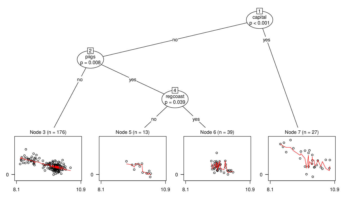
It is most striking that the speed of β-convergence is much higher for the 27 capital regions. More details about differences in the other regressors are shown in the table below. Finally, it is of interest which variables were not selected for splitting in the tree, i.e., are not associated with significant parameter instabilities: initial income, the border dummy, and Objective 1 regions, among others.
| Node | n | Partitioning | variables | Regressor | variables | |||||
|---|---|---|---|---|---|---|---|---|---|---|
| capital | piigs | regcoast | (Const.) | gdpcap0 | shgfcf | shsh | shsm | |||
| 3 | 176 | no | no | – | 0.111 (0.016) |
–0.0117 (0.0016) |
–0.0021 (0.0077) |
0.022 (0.011) |
0.0018 (0.0068) |
|
| 5 | 13 | no | yes | no | 0.161 (0.128) |
–0.0159 (0.0135) |
–0.0469 (0.0815) |
0.079 (0.059) |
–0.0234 (0.0660) |
|
| 6 | 39 | no | yes | yes | 0.073 (0.056) |
–0.0111 (0.0059) |
0.0916 (0.0420) |
0.117 (0.029) |
0.0094 (0.0218) |
|
| 7 | 27 | yes | – | – | 0.206 (0.031) |
–0.0223 (0.0029) |
–0.0075 (0.0259) |
0.041 (0.020) |
0.0528 (0.0117) |
For more details see the full manuscript. Replication materials for the entire analysis from the manuscript are available as a demo in the package:
demo("GrowthNUTS2", package = "lagsarlmtree")